Data

Data generation and data loading methods for anomalous diffusion segmentation.

Data info

We provide a set of variables with default information about the nature of the data and the default path to save it.

ROOT = Path(os.path.dirname(os.path.abspath('../')))
DATA_PATH = ROOT/"data/"
DATA_PATH.mkdir(exist_ok=True, parents=True)
FIG_PATH = DATA_PATH/"figures"
FIG_PATH.mkdir(exist_ok=True, parents=True)
MODEL_PATH = ROOT/"models"
MODEL_PATH.mkdir(exist_ok=True, parents=True)

MODEL_DATA = {
    0: {'name': 'attm', 'exps': (0.05, 1.)},
    1: {'name': 'ctrw', 'exps': (0.05, 1.)},
    2: {'name': 'fbm',  'exps': (0.05, 1.95)},
    3: {'name': 'lw',   'exps': (1.05, 2.)},
    4: {'name': 'sbm',  'exps': (0.05, 2.)}
    }
              
DEFAULT_TOKEN = -1

By default, we keep the root of the repository in ROOT, from which we define DATA_PATH=ROOT/'data' and MODEL_PATH=ROOT/'models', subsequently, we define FIG_PATH=DATA_PATH/'figures'. We use these as default paths to save and load the data, the trained models and the output figures.

Then, MODEL_DATA is a dictionary containing the information about the different anomalous diffusion models that we consider. And DEFAULT_TOKEN=-1 is the default value for the beginning of sequence token.

Data generation

To train our models, we make extensive use of simulated trajectories. The goal is to simulate realistic conditions in experiments to help our models generalize well in experimental applications.

We follow two main approaches to simulate our data depending on whether we’re working with anomalous diffusion or Brownian motion (normal diffusion).

However, the main framework is common for both. To generate trajectories with changes in diffusive behaviour, we simulate as many full trajectories as different segments we wish to have. Then, we take a sample segment of each and combine them together to obtain the resulting heterogeneous trajectory.

---

source

combine_trajectories

 combine_trajectories (datasets, dim, margin=10, random_lengths=False)

Combine the trajectories in datasets to create heterogeneous trajectories by assigning random changepoints in between.

We use pandas dataframes to store our data.

---

source

trajs2df

 trajs2df (trajectories, labels, change_points, dim, noise=None)

Stores all the trajectory information in a pandas.DataFrame.

Every row contains the information corresponding to a trajectory:

• dim: dimension of the trajecotry (1D, 2D, 3D, …) (int).
• len: trajectory length (int).
• n_cp: number of changepoints (int).
• cp: changepoint positions (torch.tensor).
• models: anomalous diffusion model of each segment (torch.tensor).
• exps: anomalous diffusion exponent of each segment (torch.tensor).
• x: trajectory (torch.tensor).
• y: models and exps for every time step (torch.tensor).
• y_mod: anomalous diffusion model for every time step (torch.tensor).
• y_exp: anomalous diffusion exponent for every time step (torch.tensor).

Anomalous diffusion segmentation dataset

We simulate anomalous diffusion trajectories following a similar recipe to the proposed in andi_datasets for the AnDi challenge.

As we specify in MODEL_DATA, there are five anomalous diffusion models that we consider, each with a different range of anomalous diffusion exponent \(\alpha\):

• Annealed transit time (ATTM) with \(\alpha\in\left[0.05, 1\right]\).
• Continuous time random walk (CTRW) with \(\alpha\in\left[0.05, 1\right]\).
• Fractional Brownian motion (FBM) with \(\alpha\in\left[0.05, 1.95\right]\).
• Lévy Walk (LW) with \(\alpha\in\left[1.05, 2\right]\).
• Scaled Brownian motion (SBM) with \(\alpha\in\left[0.05, 2\right]\).

We take \(\alpha\) values in intervals of 0.05 within the specified ranges.

Furthermore, we add localization noise in the form of white noise \(\sim\mathcal{N}(0, \sigma_{\text{noise}})\). We also show how to build a data augmentation scheme with localization noise, for which having noiseless trajectories is useful. Simply, specify noise=[0] for that.

---

source

add_localization_noise

 add_localization_noise (trajs, noise_amplitude=[0.01, 0.5, 1])

Adds white noise with standard deviation noise_amplitude.

---

source

create_andi_trajectories

 create_andi_trajectories (n_traj, max_t, dim, exponents, models,
                           noise=[0.1, 0.5, 1.0])

Creates anomalous diffusion trajectories.

For instance, we can generate a bunch of 2D FBM and SBM trajectories of 20 time steps and two levels of noise \(\sigma_{\text{noise}}=\left\{0.1, 0.5\right\}\). Furthermore, we can specify the desired values for \(\alpha\). Since both models can have a wide range of values, let’s make them purely super-diffusive \(\alpha>1\).

n_traj = 60
max_t = 20
dim = 2
exponents = np.arange(1.2, 2., 0.05)
models = [2, 4] # FBM and SBM
noise = [0.1, 0.5]
trajectories = create_andi_trajectories(n_traj, max_t, dim, exponents, models, noise=noise)

The function create_andi_trajectories tries to balance the classes for diffusion model and \(\alpha\). Usually, this results into little deviations from the specified number of trajectories. Sorry for the inconvenience!

Code

print(f"We asked for {n_traj} trajectories and got {trajectories.shape[0]}")

We asked for 60 trajectories and got 62

As this uses andi_datasets.datasets_theory to generate the trajectories, the result is an \(N\times(2+d*T)\) matrix, where \(N\) is the number of trajectories, \(d\) is the dimension, and \(T\) is the trajectory length. The first two columns contain the trajectory information: model and \(\alpha\).

trajectories.shape

(62, 42)

trajectories[:6, :2]

array([[2.  , 1.2 ],
       [2.  , 1.2 ],
       [2.  , 1.25],
       [2.  , 1.25],
       [2.  , 1.3 ],
       [2.  , 1.3 ]])

However, this method is limited to exclusively generate trajectories without changes along the way. As we mention above, we use it as a building block to generate our heterogeneous trajectories.

---

source

get_andids_fname

 get_andids_fname (n_change_points, max_t, dim, name='')

Returns standardized file name for segmentation dataset.

---

source

create_andi_segmentation_dataset

 create_andi_segmentation_dataset (n_traj:int, max_t:int=200, dim:int=1,
                                   n_change_points:int=1, models:list=[0,
                                   1, 2, 3, 4],
                                   exponents:numpy.ndarray|None=None,
                                   noise:list=[0.1, 0.5, 1.0],
                                   path:pathlib.Path|str|None=None,
                                   save:bool=True, name:str='', margin=10,
                                   random_lengths=False)

Creates a dataset for trajectory segmentation of anomalous diffusion.

	Type	Default	Details
n_traj	int		Number of trajectories
max_t	int	200	Maximum trajectory length
dim	int	1	Trajectory dimension
n_change_points	int	1	Number of changepoints in the trajectories
models	list	[0, 1, 2, 3, 4]	Diffusion models to consider
exponents	numpy.ndarray | None	None	Anomalous exponents to consider. Defaults to full range
noise	list	[0.1, 0.5, 1.0]	Noise standard deviation
path	pathlib.Path | str | None	None	Path to save the data
save	bool	True	Save or not the data
name	str		Optional name for the data set
margin	int	10
random_lengths	bool	False
Returns	DataFrame

Let’s create a segmentation dataset of a few trajectories.

n_traj = 100
df = create_andi_segmentation_dataset(n_traj, save=False)

The resulting DataFrame contains trajectories with one change point (by default), and combines all possible diffusion models and anomalous diffusion exponents.

df.columns

Index(['dim', 'len', 'n_cp', 'cp', 'models', 'exps', 'x', 'y', 'y_mod',
       'y_exp', 'noise'],
      dtype='object')

Let’s look at an example.

x0 = df.loc[0]
x0.exps, x0.models, x0.cp

(tensor([0.2500, 0.2500]), tensor([1, 2]), tensor([113]))

This trajectory changes from CTRW with \(\alpha=0.25\) to FBM with \(\alpha=0.25\) at frame 113.

Code

plt.figure(figsize=(7,4))
plt.plot(x0.x[0])
plt.vlines(x0.cp.item(), min(x0.x[0]), max(x0.x[0]), linestyles='dashed', colors='k')
plt.grid()
plt.title("Trajectory with one change point")
plt.xlabel("Time step")
plt.ylabel("Position");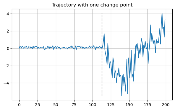

Brownian motion

We simulate Brownian motion taking the displacements as white noise with standard deviation \(\sqrt{2D\delta t}\), where \(D\) is the diffusion coefficient and \(\delta t\) is the time-step duration (we generally take \(\delta t=1\)).

---

source

brownian_motion

 brownian_motion (n_traj, max_t, D, dim=1, dt=1)

Simulate Brownian motion trajectories.

---

source

create_bm_trajectories

 create_bm_trajectories (n_traj, max_t, Ds=[1.0], shuffle=True, dim=1,
                         dt=1)

Simulate Brownian motion trajectories with various diffusion coefficients.

Similar to create_andi_trajectories, create_bm_trajectories evenly distributes the amount of trajectories for each diffusion coefficient we consider.

n_traj = 9
max_t = 5
trajectories = create_bm_trajectories(n_traj, max_t, dim=1, Ds=[1., 2.], shuffle=False)
trajectories.shape

(8, 7)

Despite only having one parameter: the diffusion coefficient \(D\), we still find two additional terms in the trajectory length which are, simply, two copies of \(D\). This is to keep a consistent formatting with the anomalous diffusion trajectories that need to store the model and \(\alpha\).

---

source

get_bmds_fname

 get_bmds_fname (n_change_points, max_t, dim, name='')

Returns consistent file name for segmentation dataset.

---

source

create_bm_segmentation_dataset

 create_bm_segmentation_dataset (n_traj:int, max_t:int=200, dim:int=1,
                                 n_change_points:int=1,
                                 Ds:collections.abc.Iterable|None=None,
                                 path:pathlib.Path|str|None=None,
                                 save:bool=True, name:str='', margin=10,
                                 random_lengths=False)

Creates a segmentation dataset to tell between diffusion coefficients.

	Type	Default	Details
n_traj	int		Number of trajectories
max_t	int	200	Maximum trajectory length
dim	int	1	Trajectory dimension
n_change_points	int	1	Number of changepoints in the trajectories
Ds	collections.abc.Iterable | None	None	Diffusion coefficients to consider defaults to logspace(-3, 3)
path	pathlib.Path | str | None	None	Path to save the data
save	bool	True	Save or not the data
name	str		Optional name for the data set
margin	int	10
random_lengths	bool	False
Returns	DataFrame

The behaviour is very similar to create_andi_segmentation_dataset. Let’s see an example.

N = 100
df = create_bm_segmentation_dataset(N, Ds=[10, 50, 100], save=False)

x0 = df.iloc[1]
x0.exps, x0.cp

(tensor([100.,  10.]), tensor([54]))

The trajectory changes from \(D=100\) to \(D=10\) at the 54th time-step.

Code

plt.figure(figsize=(7,4))
plt.plot(x0.x[0])
plt.vlines(x0.cp.item(), min(x0.x[0]), max(x0.x[0]), linestyles='dashed', colors='k')
plt.grid()
plt.title("Trajectory with one change point")
plt.xlabel("Time step")
plt.ylabel("Position");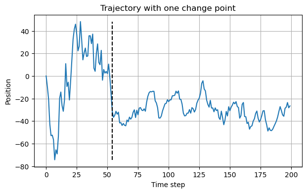

ATTM trajectories

Annealed transit time (ATTM) is an anomalous diffusion model consisting of piecewise normal diffusion. Every segment has a random diffusion coefficient \(D\) drawn with probability \[P(D) = \frac{D^{\sigma - 1}\exp(-D/b)}{b^\sigma\Gamma(\sigma)}\,,\] with parameters \(\sigma\) and \(b\). The residence time in each diffusive state, \(\tau\), depends on the magnitude of the diffusion coefficient: \[P_\tau(\tau|D)=\frac{D^\gamma}{k}\exp(-\tau D^\gamma/k)\,,\] with parameters \(\gamma\) and \(k\). The parameters \(\sigma\) and \(\gamma\) in these distributions determine the anomalous exponent \(\alpha=\sigma/\gamma\), whenever \(\sigma<\gamma<\sigma+1\). Thus, for every \(\alpha\) there are infinitely many valid combinations of \(\sigma, \,\gamma\).

In andi_datasets, these parameters are randomly sampled given a fixed \(\alpha\). Here, we wish to extract \(\sigma\) and \(\gamma\) and, thus, we need a consistent way to simulate ATTM trajectories with those parameters fixed.

Note

In our work, we use ATTM trajectories to show how to characterize anomalous diffusion directly from changes in normal diffusion.

---

source

create_fixed_attm_trajs

 create_fixed_attm_trajs (n_traj, max_t, sigma, gamma)

Creates 2-D ATTM trajectories with fixed sigma and gamma.

Let’s generate some ATTM trajectories with fixed \(\sigma=0.3\) and \(\gamma=0.4\), meaning that \(\alpha=0.75\).

n_traj = 2
max_t = 15
sigma, gamma = 0.3, 0.4
trajs, ds = create_fixed_attm_trajs(n_traj, max_t, sigma, gamma)

Code

fig, axes = plt.subplots(nrows=1, ncols=2, figsize=(7, 3), constrained_layout=True)
axes[0].plot(trajs[0].T)
axes[0].set_xlabel("Time", fontsize=16)
axes[0].set_ylabel("Position", fontsize=16)
axes[0].tick_params(labelsize=14)

axes[1].semilogy(ds[0])
axes[1].set_xlabel("Time", fontsize=16)
axes[1].set_ylabel("D", fontsize=16)
axes[1].tick_params(labelsize=14)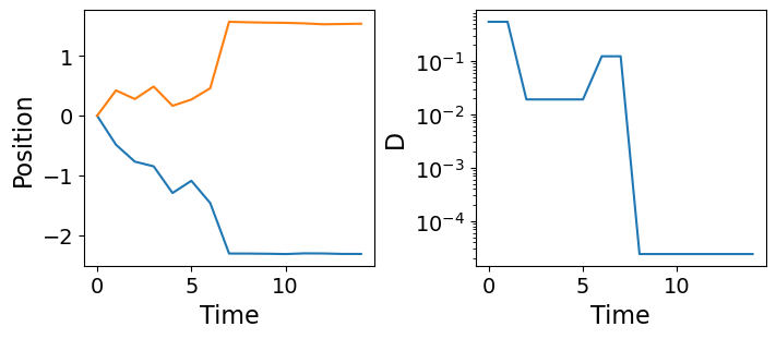

Datasets with variable number of change points

So far we have shown how to build data sets with a fixed number of changepoints. In order to make a dataset that contains a variable number of change points, we can simply combine several of those in a smart way.

This will make our models much more robust and allow us to generalize better to experimental data with an arbitrary number of changes along the trajectories.

---

source

combine_datasets

 combine_datasets (datasets, shuffle=True)

Combines data sets together.

Example: Brownian motion

With this code, we have generated the main test set of Brownian motion trajectories to validate our models.

N_per_set = 12000
max_t = 200
dim = 2
Ds = np.logspace(-3, 3, 1000) 
cps = [1, 2, 3, 4]
# Choose a function to create datasets either brownian motion or anomalous diffusion
ds_fun = partial(create_bm_segmentation_dataset,
                 max_t=max_t, dim=dim, Ds=Ds, save=False)

datasets = [ds_fun(N_per_set, n_change_points=n_cp) for n_cp in cps]
dataset = combine_datasets(datasets)

save_path = DATA_PATH/get_bmds_fname(f'{min(cps)}_to_{max(cps)}', max_t, dim, 'test')
dataset.to_pickle(save_path)

Example: anomalous diffusion

With this code, we have generated the main test set of anomalous diffusion trajectories to validate our models.

N_per_set = 12500
max_t = 200
dim = 2 
cps = [1, 2, 3, 4]
# Choose a function to create datasets either brownian motion or anomalous diffusion
ds_fun = partial(create_andi_segmentation_dataset,
                 models=models, max_t=max_t, dim=dim, noise=[0.], save=False)

datasets = [ds_fun(N_per_set, n_change_points=n_cp) for n_cp in cps]
dataset = combine_datasets(datasets)

save_path = DATA_PATH/get_andids_fname(f'{min(cps)}_to_{max(cps)}', max_t, dim, 'test')
dataset.to_pickle(save_path)

Validation with AnDi

It is useful to validate our models over the AnDi challenge data sets to compare them with the top performing models of the challenge.

By default, we asume the data is in DATA_PATH/andi_val_{task_number}.

---

source

load_andi_data

 load_andi_data (dim=1, task=1, path=None)

Loads data from AnDi.

df = load_andi_data(dim=2)
df.shape

(10000, 4)

df.head(2)

	dim	len	x	y
0	2	200	[[tensor(0.), tensor(-0.5156), tensor(-0.8383), tensor(-1.4615), tensor(-1.7552), tensor(-1.6362), tensor(-1.4192), tensor(-1.3548), tensor(-1.2144), tensor(-1.7406), tensor(-1.6199), tensor(-1.4474), tensor(-0.2902), tensor(0.5447), tensor(0.5666), tensor(0.1618), tensor(-0.1004), tensor(-0.1377), tensor(-1.1998), tensor(-1.9200), tensor(-3.1992), tensor(-4.4678), tensor(-5.7045), tensor(-6.3007), tensor(-6.6895), tensor(-7.5415), tensor(-7.9907), tensor(-9.3120), tensor(-10.1935), tensor(-10.5246), tensor(-11.5122), tensor(-12.5124), tensor(-13.6076), tensor(-13.9701), tensor(-14.3846), ...	[]
1	2	200	[[tensor(0.), tensor(1.8434), tensor(2.5901), tensor(3.3360), tensor(3.3675), tensor(5.1754), tensor(6.7046), tensor(6.5266), tensor(5.5823), tensor(4.2652), tensor(2.6675), tensor(2.0960), tensor(1.3606), tensor(-0.0349), tensor(-1.4965), tensor(-0.4068), tensor(-1.8796), tensor(-1.7324), tensor(-1.8430), tensor(-0.4918), tensor(0.8988), tensor(1.1704), tensor(2.8995), tensor(3.4126), tensor(3.3071), tensor(4.3777), tensor(4.9901), tensor(6.3406), tensor(7.1728), tensor(8.1412), tensor(9.1267), tensor(9.0713), tensor(9.1243), tensor(11.2437), tensor(12.1926), tensor(12.3969), tensor(12.98...	[]

DataLoaders

Data loaders are essential to train our machine learning models. We provide functions that load the data and return appropiate fastai.DataLoaders for the segmentation tasks.

---

source

load_dataset

 load_dataset (n_change=1, max_t=200, dim=1, name='', path=None, bm=False)

Loads dataset according to n_change, max_t and dim or straight from path.

---

source

get_segmentation_dls

 get_segmentation_dls (target:str='y_mod', models:list|None=None,
                       exps:collections.abc.Iterable|None=None,
                       size:int|None=None, bs:int=128,
                       split_pct:float=0.2, shuffle:bool=True,
                       tfm_y:collections.abc.Callable|None=None,
                       n_change:int|str=1, bm:bool=False, max_t=200,
                       dim=1, name='', path=None)

Obtain DataLoaders from dataset filtered by models and exps to predict target.

	Type	Default	Details
target	str	y_mod	Task target y_mod, y_exp or y for both.
models	list | None	None	List of models to consider. Defaults to all.
exps	collections.abc.Iterable | None	None	List of anomalous exponents to consider. Deafults to all.
size	int | None	None	Maximum data set size. Defaults to full data set.
bs	int	128	Batch size.
split_pct	float	0.2	Validation set split percentage from training data.
shuffle	bool	True	Shuffle the dataset.
tfm_y	collections.abc.Callable | None	None	Transformation to apply to the target, e.g., torch.log10.
n_change	int | str	1	Number of changes in the trajectories, e.g., ‘1_to_4’.
bm	bool	False	Is it Brownian motion (False for anomalous diffusion)
max_t	int	200
dim	int	1
name	str
path	NoneType	None
Returns	DataLoaders

This is the main function to obtain DataLoaders for a segmentation task. These provide the trajetories with their corresponding labels at every time step.

Let’s see an example for a classification task (setting target='y_mod'). We take a sub-sample of the dataset of size=100 with a batch size bs=4.

seg_dls = get_segmentation_dls(size=100, bs=4)
x, y = seg_dls.one_batch()
x.shape, y.shape

(torch.Size([4, 200, 1]), torch.Size([4, 200]))

In this example, we have 1-dimensional trajectories with 200 time steps. Thus, the target is also 200 frames long.

x[0, :5], y[0, :5]

(tensor([[0.0000],
         [3.3110],
         [4.2102],
         [7.4056],
         [4.6176]]),
 tensor([3, 3, 3, 3, 3]))

---

source

SegmentationTransform

 SegmentationTransform (target='y_mod', n_class=5, init_token=None)

Delegates (__call__,decode,setup) to (encodes,decodes,setups) if split_idx matches

---

source

get_transformer_dls

 get_transformer_dls (target='y_mod', dim=1, n_change=1, max_t=200,
                      valid_pct=0.2, models=None, exps=None, size=None,
                      data_path=None, init_token=None, bs:int=64,
                      shuffle_train:bool=None, shuffle:bool=True,
                      val_shuffle:bool=False, n:int=None,
                      path:str|Path='.', dl_type:TfmdDL=None,
                      dl_kwargs:list=None, device:torch.device=None,
                      drop_last:bool=None, val_bs:int=None)

Obtain DataLoaders from filtered dataset prepared for transformer training.

	Type	Default	Details
target	str	y_mod
dim	int	1
n_change	int	1
max_t	int	200
valid_pct	float	0.2
models	NoneType	None
exps	NoneType	None
size	NoneType	None
data_path	NoneType	None
init_token	NoneType	None
bs	int	64	Batch size
shuffle_train	bool	None	(Deprecated, use shuffle) Shuffle training DataLoader
shuffle	bool	True	Shuffle training DataLoader
val_shuffle	bool	False	Shuffle validation DataLoader
n	int	None	Size of Datasets used to create DataLoader
path	str | Path	.	Path to put in DataLoaders
dl_type	TfmdDL	None	Type of DataLoader
dl_kwargs	list	None	List of kwargs to pass to individual DataLoaders
device	torch.device	None	Device to put DataLoaders
drop_last	bool	None	Drop last incomplete batch, defaults to shuffle
val_bs	int	None	Validation batch size, defaults to bs

Transformer data loaders provide three items: raw trajectory (src), one-hot encoding of labels (tgt) and the labels to compute the loss. These are mainly intended for pointwise classification tasks, such as inferring the anomalous diffusion model behind the simulation. Otherwise, the one-hot-encoding does not make much sense.

tfm_dls = get_transformer_dls(size=100, bs=4)

x, y_one_hot, y = tfm_dls.one_batch()
x.shape, y_one_hot.shape, y.shape

(torch.Size([4, 200, 1]), torch.Size([4, 200, 5]), torch.Size([4, 200]))

idx = 0
x[idx, :5], y_one_hot[idx, :5], y[idx, :5]

(tensor([[ 0.0000],
         [-0.0976],
         [-0.0456],
         [ 0.0426],
         [ 0.0395]], device='cuda:0'),
 tensor([[-1., -1., -1., -1., -1.],
         [ 0.,  0.,  1.,  0.,  0.],
         [ 0.,  0.,  1.,  0.,  0.],
         [ 0.,  0.,  1.,  0.,  0.],
         [ 0.,  0.,  1.,  0.,  0.]], device='cuda:0'),
 tensor([2, 2, 2, 2, 2], device='cuda:0'))

---

source

get_andi_valid_dls

 get_andi_valid_dls (bs=128, pct=1, dim=1, task=1, path=None)

Obtain DataLoaders from AnDi challenge validation data.

When validating on the AnDi challenge data, in some cases, it may be convenient to work with DataLoaders instaed of DataFrames, which can be obtained through load_andi_data. These are mainly intended to test our models. Thus, notice that the split percentage for train/validation is set to 100% validation by default.

andi_dls = get_andi_valid_dls(dim=2)
x, y = andi_dls.valid.one_batch()
x.shape, y.shape

(torch.Size([128, 200, 2]), torch.Size([128, 0]))

x[0, :5]

tensor([[ 0.0000,  0.0000],
        [-0.5156,  0.5875],
        [-0.8383,  0.5096],
        [-1.4615,  0.5320],
        [-1.7552,  0.4109]])