Models

Architectures for trajectory segmentation.

Utility layers

---

source

tfm_encoder

 tfm_encoder (dim, n_head=1, n_layers=8, dim_ff=1024, dropout=0.1,
              activation='relu')

Creates a nn.TransformerEncoder.

---

source

ConcatPooling

 ConcatPooling (dim=-1)

Perform max and average pool over dim. Outputs [avg_pool, max_pool].

---

source

Transpose

 Transpose (dims)

Transposition layer of dims.

---

source

Normalization

 Normalization (dim=-1)

Z-Normalization over the designated dimension.

---

source

get_act

 get_act (vocab_sz, yrange=(0, 2.05))

Provides a sigmoid or softmax activation according to inferring the task (regression or classification) from vocab_sz.

Dense layers

---

source

LinBnDropTrp

 LinBnDropTrp (n_in, n_out, bn=True, p=0.0, trp=(2, 1), act=None, ndim=1)

Linear layer with batch norm, dropout and transposition.

---

source

Classifier

 Classifier (dims, ps, final_act=False, yrange=None, trp=(2, 1))

Dense classifier.

We use the Classifier at the end of most of our models. It is comprised of LinBnDropTrp layers that allow us to obtain the desired output dimension for any task. Furthermore, we can specify whether to apply a final activation function through final_act. In classification tasks with pytorch, where we use CrossEntropyLoss or fastai’s CrossEntropyLossFlat, we do not want to apply the softmax activation function to the logits before passing them to the loss function.

Self-attention-based models

Extracting pointwise properties of a sequence can be understood as a translation task. Thus, it is natural to tackle the problem using a transformer or other purely self-attention-based architectures. Here, we provide a full Transformer (encoder + decoder), and an encoder-only model EncoderClassifier.

---

source

Transformer

 Transformer (dim, n_class=5, nhead_enc=1, nhead_dec=1,
              num_encoder_layers=6, num_decoder_layers=6, dim_ff=2048,
              dropout=0.1, activation='relu')

Transformer architecture.

The Transformer implements a basic transformer architecture as introduced in Attention is all you need from Vaswani, et. al., in 2017.

Let’s see an example of how to train a transformer to perform a segmentation task of the anomalous diffusion model in heterogeneous trajectories.

# Data loaders
tfm_dls = get_transformer_dls(bs=128)
tfm_dls.device = default_device()
# Model
my_tf = Transformer(1, num_encoder_layers=4, num_decoder_layers=4, dim_ff=500)
my_tf.to(default_device())
# Learner
learn = Learner(tfm_dls, my_tf, loss_func=CrossEntropyLossFlat(), model_dir=MODEL_PATH)

learn.fit_one_cycle(15, lr_max=1e-2)

epoch	train_loss	valid_loss	time
0	0.081026	0.063063	00:41
1	0.047181	0.045920	00:40
2	0.044656	0.043783	00:41
3	0.043903	0.043491	00:40
4	0.043756	0.043521	00:41
5	0.043616	0.043354	00:41
6	0.043514	0.043158	00:40
7	0.043429	0.043019	00:41
8	0.043339	0.043081	00:41
9	0.043207	0.042961	00:41
10	0.043100	0.042880	00:41
11	0.043028	0.042799	00:41
12	0.042846	0.042705	00:40
13	0.042833	0.042656	00:41
14	0.042852	0.042683	00:41

Warning

The task is particularly bad conditioned for a naive transformer training such as this one. The loss does get low, but it is mainly because the model learns to predict whatever the previous token was, so be careful!

In these segmentation tasks over piecewise constant segments, the target may look like \([2,2,2,2,2,1,1,1,1,1]\). With such naive training scheme, the transformer learns to replicate whatever the last digit is and it fails to find the changepoints. Let’s have a look at some predictions.

x, y_one_hot, y = dls.one_batch()
learn.model.eval()
preds, pred_one_hot, outs = learn.model.segment(x)

preds[:10, :10]

tensor([[4, 4, 4, 4, 4, 4, 4, 4, 4, 4],
        [4, 4, 4, 4, 4, 4, 4, 4, 4, 4],
        [4, 4, 4, 4, 4, 4, 4, 4, 4, 4],
        [4, 4, 4, 4, 4, 4, 4, 4, 4, 4],
        [4, 4, 4, 4, 4, 4, 4, 4, 4, 4],
        [4, 4, 4, 4, 4, 4, 4, 4, 4, 4],
        [4, 4, 4, 4, 4, 4, 4, 4, 4, 4],
        [4, 4, 4, 4, 4, 4, 4, 4, 4, 4],
        [4, 4, 4, 4, 4, 4, 4, 4, 4, 4],
        [4, 4, 4, 4, 4, 4, 4, 4, 4, 4]], device='cuda:0')

y[:10, :10]

tensor([[4, 4, 4, 4, 4, 4, 4, 4, 4, 4],
        [0, 0, 0, 0, 0, 0, 0, 0, 0, 0],
        [2, 2, 2, 2, 2, 2, 2, 2, 2, 2],
        [3, 3, 3, 3, 3, 3, 3, 3, 3, 3],
        [1, 1, 1, 1, 1, 1, 1, 1, 1, 1],
        [2, 2, 2, 2, 2, 2, 2, 2, 2, 2],
        [3, 3, 3, 3, 3, 3, 3, 3, 3, 3],
        [0, 0, 0, 0, 0, 0, 0, 0, 0, 0],
        [0, 0, 0, 0, 0, 0, 0, 0, 0, 0],
        [4, 4, 4, 4, 4, 4, 4, 4, 4, 4]], device='cuda:0')

The model has correctly predicted the label for the first segment: 4 corresponding to SBM. However, it has then proceeded to replicate the label over the whole trajectory. You’ll need some extra tricks to train this :)

---

source

PositionalEncoding

 PositionalEncoding (d_model, dropout=0.1, max_len=10000)

Same as nn.Module, but no need for subclasses to call super().__init__

Transformers see the trajectories all at once without any notion of distance between the points. Here, we implement a positional encoding based on the addition of sines and cosines to the data, as introduced in the original paper.

pe = PositionalEncoding(14, max_len=100)
pos_enc = pe.pos_enc.squeeze()

Code

fontsize, ticksize = 20, 15
fig, axes = plt.subplots(2, sharex=True, figsize=(14, 8))
for sin, cos in zip(pos_enc.T[::2], pos_enc.T[1::2]):
    axes[0].plot(sin)
    axes[1].plot(cos)

axes[1].set_xlabel("Position", fontsize=fontsize)
axes[0].set_ylabel("sin activation", fontsize=fontsize)
axes[1].set_ylabel("cos activation", fontsize=fontsize)
for ax in axes:
    ax.grid()
    ax.tick_params(labelsize=ticksize)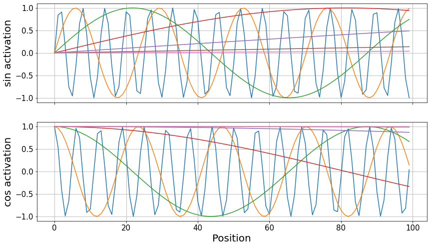

---

source

EncoderClassifier

 EncoderClassifier (dim, length=200, n_class=5, nhead_enc=1,
                    num_encoder_layers=6, dim_ff=2048, dropout=0.1,
                    activation='relu', linear_layers=[1024], ps=None,
                    yrange=(0, 2.05), final_act=False, trp=(2, 1))

Transformer encoder with a linear classifier.

dls = get_segmentation_dls()
dls.device = default_device()
enc = EncoderClassifier(1, num_encoder_layers=12, dim_ff=1024)
enc.to(default_device())
learn = Learner(dls, enc, loss_func=CrossEntropyLossFlat(), model_dir=MODEL_PATH)

learn.fit_one_cycle(5, lr_max=1e-1)

epoch	train_loss	valid_loss	time
0	1.611631	1.609615	00:58
1	1.611847	1.613333	00:58
2	1.611033	1.609803	00:59
3	1.609777	1.609575	00:59
4	1.609749	1.609633	01:00

Combined convolutional and self-attention models

Convolutional models have seen great success characterizing diffusion trajectories, specially combined with recurrent neural networks, as seen in the AnDi challenge paper. We provide a few models that combine convolutional feature extractors with self-attention mechanisms.

---

source

ConvAttn

 ConvAttn (dim, n_class=5, conv_dims=[64, 128, 128], nhead_enc=1,
           num_encoder_layers=6, dim_ff=2048, dropout=0.1,
           linear_layers=[128], activation='relu', yrange=(0, 2.05))

Convolution layers with a transformer encoder.

ConvAttn is built out of basic convolutional layers that act as an embedding for a transformer encoder. There is a dense Classifier at the end that achieves the desired output dimensions.

Performing a diffusion model segmentation task is the most straightforward, simply specify the trajectory dimension, which defaults to dim=1 in the dataloaders and provide the appropiate loss function CrossEntropyLossFlat.

dls = get_segmentation_dls()
dls.device = default_device()
model = ConvAttn(2, conv_dims=[64, 128, 128], num_encoder_layers=8, dim_ff=512, nhead_enc=8, linear_layers=[])
model.to(default_device())
learn = Learner(dls, model, loss_func=CrossEntropyLossFlat(), model_dir=MODEL_PATH)

For anomalous exponent segmentation, we must specify the target target='y_exp' as well as provide the corresponding loss function, either L1LossFlat or MSELossFlat. Don’t forget to provide the model with the proper number of classes n_class=1.

dls = get_segmentation_dls(target='y_exp')
dls.device = default_device()
model = ConvAttn(1, n_class=1, conv_dims=[32, 64, 128, 256], num_encoder_layers=8, dim_ff=512, nhead_enc=8, linear_layers=[])
model.to(default_device())
learn = Learner(dls, model, loss_func=L1LossFlat(), model_dir=MODEL_PATH)

To train, we simply call learn.fit_one_cycle.

---

source

XResBlocks

 XResBlocks (block, layers, expansion=1, p=0.0, c_in=1, n_out=1000,
             stem_szs=(32, 32, 64), block_szs=None, widen=1.0, ndim=1,
             ks=3, stride=2, sa=False, stem_stride=False, act_cls=<class
             'torch.nn.modules.activation.ReLU'>, groups=1,
             reduction=None, nh1=None, nh2=None, dw=False, g2=1,
             sym=False, norm_type=<NormType.Batch: 1>, pool=<function
             AvgPool>, pool_first=True, padding=None, bias=None,
             bn_1st=True, transpose=False, init='auto', xtra=None,
             bias_std=0.01, dilation:Union[int,Tuple[int,int]]=1,
             padding_mode:str='zeros', device=None, dtype=None)

XResNet block.

XResBlocks follow the XResNet architecture to build a convolutional neural network feature extractor.

The blocks start with an initial purely-convolutional stem. Then, every subsequent block consists of two convolutional layers with a skip connection or identity path. The identity paths have a single convolutional layer with kernel size 1 to match the channel dimension of their corresponding convolutional paths.

---

source

XResAttn

 XResAttn (dim, n_class=5, conv_blocks=[1, 1], block=<class
           'fastai.layers.ResBlock'>, block_szs=[64, 128], nhead_enc=1,
           n_encoder_layers=6, dim_ff=2048, dropout=0.1, pos_enc=True,
           linear_layers=[128], activation='relu', norm=True, yrange=(0,
           2.05), expansion=1, p=0.0, c_in=1, n_out=1000, stem_szs=(32,
           32, 64), widen=1.0, ndim=1, ks=3, stride=2, sa=False,
           stem_stride=False, act_cls=<class
           'torch.nn.modules.activation.ReLU'>, groups=1, reduction=None,
           nh1=None, nh2=None, dw=False, g2=1, sym=False,
           norm_type=<NormType.Batch: 1>, pool=<function AvgPool>,
           pool_first=True, padding=None, bias=None, bn_1st=True,
           transpose=False, init='auto', xtra=None, bias_std=0.01,
           dilation:Union[int,Tuple[int,int]]=1, padding_mode:str='zeros',
           device=None, dtype=None)

Xresnet blocks with attention at the end.

	Type	Default	Details
dim
n_class	int	5
conv_blocks	list	[1, 1]
block	PrePostInitMeta	ResBlock
block_szs	list	[64, 128]
nhead_enc	int	1
n_encoder_layers	int	6
dim_ff	int	2048
dropout	float	0.1
pos_enc	bool	True
linear_layers	list	[128]
activation	str	relu
norm	bool	True
yrange	tuple	(0, 2.05)
expansion	int	1
p	float	0.0
c_in	int	1
n_out	int	1000
stem_szs	tuple	(32, 32, 64)
widen	float	1.0
ndim	int	1
ks	int	3
stride	int	2
sa	bool	False
stem_stride	bool	False
act_cls	type	ReLU
groups	int	1
reduction	NoneType	None
nh1	NoneType	None
nh2	NoneType	None
dw	bool	False
g2	int	1
sym	bool	False
norm_type	NormType	NormType.Batch
pool	function	AvgPool
pool_first	bool	True
padding	NoneType	None
bias	NoneType	None
bn_1st	bool	True
transpose	bool	False
init	str	auto
xtra	NoneType	None
bias_std	float	0.01
dilation	Union	1
padding_mode	str	zeros	TODO: refine this type
device	NoneType	None
dtype	NoneType	None

XResAttn is an evolution of ConvAttn in which we replace the basic convolutional layer by XResBlocks.

dim = 2
dls = get_segmentation_dls(dim=dim, target='y_exp', size=10000)
dls.device = default_device()
model = XResAttn(dim, n_class=1, stem_szs=(32,), conv_blocks=[1, 1], block_szs=[64, 128], 
                 n_encoder_layers=6, dim_ff=512, nhead_enc=8, linear_layers=[])
model.to(default_device())
learn = Learner(dls, model, loss_func=L1LossFlat(), model_dir=MODEL_PATH)

learn.fit_one_cycle(15, lr_max=2e-4)

epoch	train_loss	valid_loss	time
0	0.351831	0.341731	05:52
1	0.317376	0.313373	05:53
2	0.296154	0.291456	05:53
3	0.276105	0.274482	05:53
4	0.265737	0.263980	05:53
5	0.256997	0.253854	05:53
6	0.245702	0.243755	05:53
7	0.243005	0.237430	05:53
8	0.235679	0.235492	05:53
9	0.231861	0.231436	05:53
10	0.231640	0.229545	05:53
11	0.225968	0.227001	05:53
12	0.223144	0.226924	05:54
13	0.223188	0.226133	05:54
14	0.219965	0.225446	05:53

---

source

LogXResAttn

 LogXResAttn (dim, n_class=5, conv_blocks=[1, 1], block=<class
              'fastai.layers.ResBlock'>, block_szs=[64, 128], nhead_enc=1,
              n_encoder_layers=6, dim_ff=2048, dropout=0.1, pos_enc=True,
              linear_layers=[128], activation='relu', norm=True,
              yrange=(0, 2.05), **kwargs)

Xresnet blocks with attention at the end. t takes the logarithm of the displacements.

The LogXresAttn model extracts the displacements of the input trajectory and works with their logarithm, rather than with the raw positional data. This allows it to seamlessly deal with trajectories that display diffusion coefficients across several orders of magnitude that could otherwise be lost in the numerical precision.

Note

Since LogXresAttn works with the trajectory displacements, its output is a prediction for every displacement. While this is more physically meaningful, we need to take into account that the output dimension will be smaller (\(N-1\) displacements for \(N\) points).

U-net

U-nets were originally conceived to perform image segmentation. Therefore, they are particularly well-suited for the trajectory segmentation task.

We provide a dynamic U-net that takes the backbone of a model and transforms it into the U-like architecture.

---

source

icnr_init_general

 icnr_init_general (x, scale=2, init=<function kaiming_normal_>)

Generalized version of icnr_init.

---

source

GeneralPixleShuffle

 GeneralPixleShuffle (upscale_factor)

Generalized Pixle Shuffle to work with any data dimensionality.

---

source

PixelShuffleUpsampling

 PixelShuffleUpsampling (ni, nf=None, scale=2, ndim=2, blur=False,
                         norm_type=<NormType.Weight: 3>, act_cls=<class
                         'torch.nn.modules.activation.ReLU'>)

Updample by scale from ni filters to nf using GeneralPixleShuffle.

---

source

UnetBlock

 UnetBlock (up_in_c, x_in_c, hook, ndim=1, final_div=True, blur=False,
            act_cls=<class 'torch.nn.modules.activation.ReLU'>,
            self_attention=False, init=<function kaiming_normal_>,
            norm_type=None, ks=3, stride=1, padding=None, bias=None,
            bn_1st=True, transpose=False, xtra=None, bias_std=0.01,
            dilation:Union[int,Tuple[int,int]]=1, groups:int=1,
            padding_mode:str='zeros', device=None, dtype=None)

A quasi-UNet block using pixel shuffle upsampling.

A key element of the U-net is the upsmapling branch. We do it by stacking UnetBlocks that perform convolution-based upsampling with pixel shuffle. We implement a PixelShuffleUpsampling layer that uses our GeneralPixleShuffle, which is a generalized version of the original pixel shuffle.

To build the downsampling branch, we take the desired architecture and we pass a dummy input through it to extract relevant information, such as the points at which dimensions change, which then need to be connected to the upsampling branch.

---

source

dummy_eval

 dummy_eval (m, size=(64, 64))

Evaluate m on a dummy input of a certain size

---

source

in_channels

 in_channels (m)

Return the shape of the first weight layer in m.

---

source

model_sizes

 model_sizes (m, size=(64, 64))

Pass a dummy input through the model m to get the various sizes of activations.

---

source

get_sz_change_idxs

 get_sz_change_idxs (sizes)

Get the indexes of the layers where the size of the activation changes.

---

source

ResizeToOrig

 ResizeToOrig (mode='nearest')

Merge a shortcut with the module result by adding or concatenating them if dense=True.

---

source

AttnDynamicUnet

 AttnDynamicUnet (encoder, n_out, img_size, ndim=1, num_encoder_layers=6,
                  nhead_enc=8, dim_ff=1024, p=0.1, act='relu', blur=False,
                  blur_final=True, self_attention=False, y_range=None,
                  last_cross=True, bottle=False, act_cls=<class
                  'torch.nn.modules.activation.ReLU'>, init=<function
                  kaiming_normal_>, norm_type=None, **kwargs)

Create a U-Net from a given architecture.

AttnDynamicUnet builds a U-net like architecture from a given architecture (encoder). The input encoder conforms the downsampling branch, then, we add a convolution and a transformer encoder at the center (bottom of the U), and build the upsampling branch with UnetBlocks that have skip connections wherever the dimension in the encoder changes.

---

source

UnetModel

 UnetModel (encoder, n_class, img_size, nf=64, linear_layers=[128], p=0.1,
            y_range=(0, 2.05), ndim=1, num_encoder_layers=6, nhead_enc=8,
            dim_ff=1024, act='relu', blur=False, blur_final=True,
            self_attention=False, last_cross=True, bottle=False,
            act_cls=<class 'torch.nn.modules.activation.ReLU'>,
            init=<function kaiming_normal_>, norm_type=None)

U-net with a final dense layer.

UnetModel uses AttnDynamicUnet to build a U-net from a desired architecture and appends a Classifier at the end to obtain the desired output dimension for the task.

For example, we can easily build a U-net with an XResNet encoder to infer the anomalous diffusion exponent \(\alpha\) at every time step of the input trajectories.

dls = get_segmentation_dls(target='y_exp')
dls.device = default_device()
encoder = XResBlocks(ResBlock, [1, 2, 1], c_in=1, stem_szs=(32,), block_szs=[64, 128, 256])
umodel = UnetModel(encoder, 1, (200,), num_encoder_layers=4, dim_ff=512, linear_layers=[], y_range=(0, 2.05))
umodel.to(default_device())
ulearn = Learner(dls, umodel, loss_func=L1LossFlat(), model_dir=MODEL_PATH)

ulearn.fit_one_cycle(15, lr_max=1e-3)

epoch	train_loss	valid_loss	time
0	0.353012	0.344957	00:35
1	0.335089	0.334739	00:35
2	0.332037	0.327504	00:35
3	0.324102	0.323693	00:36
4	0.317840	0.316003	00:36
5	0.312131	0.314038	00:36
6	0.309137	0.310193	00:35
7	0.308097	0.305047	00:35
8	0.303723	0.304123	00:36
9	0.299942	0.302303	00:36
10	0.299658	0.300621	00:36
11	0.297696	0.300281	00:36
12	0.293374	0.299450	00:36
13	0.292193	0.299131	00:36
14	0.290734	0.299084	00:36