Generative models

Introduction to unsupervised learning and generative models

1 Unsupervised learning

Unsupervised learning consists on capturing rich patterns in the data in a label-free approach. This is opposed to the supervised learning scheme, in which we have a data set comprised of labeled samples \(\left\{\mathbf{x}, y\right\}\) and we try to approximate the function \(f(x)\approx y(x)\).

In unsupervised learning, even though we follow label-free approaches, what we would consider labels can some times be part of the data corpus.

We can split deep unsupervised learning in two main categories: generative and self-superivsed learning, although the line is often blurred. In generative learning, we try to recreate the data distribution. This allows us to generate new data points that are likely to belong to the original data set, and often even know the probability to observe them. In self-supervised learning, we instead focus on finding different representations of the data. These are often useful to accomplish other tasks, compress the information, etc.

Indeed, in some cases, the resulting models can accomplish downstream tasks without having been trained to perform them explicitly. For example, the generative model GPT-3 Brown et al. (2020) is a language model, as we saw earlier in the course, that can perform question answering tasks (among others) without any further specific training for it. Or the self-supervised vision model DINO Caron et al. (2021) can extract segmentation masks from images (see Figure 1), such as the ones we saw in the computer vision example tasks.

Figure 1: Self-supervised segmentation masks from DINO

Unsupervised methods have gathered a lot of attention in scientific applications, as they can help us extract physically relevant information from experimental data Iten et al. (2020). Actually, in science, some times we do not even know what to look for in the data! For example, supose that we want to characterize a complex quantum system. To do so, we need to consider all the possible phases the system can be and devise appropiate order parameters to test whether they exist and find the phase transitions. With self-supervised methods, we can find different data representation schemes for specific regions of the phase diagram. This way, we can explore the phase diagram autonomously to find where the phase transitions may be in our system Kottmann et al. (2020).

Most of the recent advances in the machine learning (ML) field have been mainly due to massive scaling, both in terms of the model size and the amount of data. This has relied heavily in the vast amount of unlabeled data that exists in the internet. Think about it, for every cat image in every appropiately labeled data set we can find, how many unlabeled cat images and videos are in the internet? The current state-of-the-art practice in many ML applications consists on training an unsupervised model with huge amounts of unlabeled data and, then, leveraging its knowledge to accomplish the desired task. We saw this procedure when we adapted our language model trained on wikipedia to write movie reviews, and then, we used it to classify them.

This process is akin to the way humans learn. Our brain processes a continuous stream of unlabeled data containing rich information about our environment. Furthermore, we never process the exact same information twice, as there are no two instances of our life that are exactly the same. This allows us to generalize extremely well and make the most out of the relatively scarse labeled data we have access to. For example, given a single stegosaurus image, we can immediately recognize this dinosaur species anywhere else, with any camera angle, any art-style, and even with partial information (e.g. just a part of the dinosaur).

Thus, unsupervised learning is essential for the entire ML field and it is specially promising in scientific applications.

2 Generative modeling

Here, we focus in generative learning. As we have briefly mentioned before, it consists on learning the data distribution to generate new samples. This is extremely powerful both on its own, since high-quality new samples can be very valuable, and in combination with other tools to tackle downstream tasks, as in the movie review example.

There are many data generation approaches that we can consider. The most straightforward one is to simply generate samples that are similar to the traning ones, such as face images or digits. We can also have conditioned synthesis, such as generating an audio signal from a text prompt that can be conditioned to a specific speaker voice (e.g. WaveNet). This involves all sorts of translation tasks, where we write text from a sample fragment, generate a new image from a reference one (see the emblematic horse-to-zebra example), or even create a video from a text fragment!

Note

This is a very broad field and here we just show a hand full of representative examples.

2.1 Learning the data probability distribution

The task is to learn the underlying distribution \(p_{\text{data}}(x_i)\) given a data set \(\left\{x_i\right\}\). We can do this either finding a model to approximate the probability distribution, \(p_\theta(x_i)\approx p_{\text{data}}\), and then sample from it, or by training a model to generate new samples and then estimate \(p_{\text{data}}\).

Note

Just because we can compute the probability it does not mean that we can sample easily and vice versa. In general, there is a trade-off between sampling and computing the probability.

To illustrate the main concepts, we will consider a toy model with samples \(\left\{x_i\right\}\) drawn from a mixture of two Gaussian distributions: \(\mathcal{N}_0(\mu_0,\sigma_0)\) and \(\mathcal{N}_1(\mu_1,\sigma_1)\). A common way to model mixture models is through a multinoulli distribution that assigns the probability to sample from each of the possible modes. Since in this case we only have two modes, we can use a Bernoulli distribution instead with \(p(x)=\phi^x(1-\phi)^{1-x}\), meaning that \(p(x=1) = \phi\) and \(p(x=0) = 1-\phi\).

Exercise

Define a function to sample from the Gaussian mixture described above. As input, it should take the desired number of samples GaussianMixture.sample(self, n_samples).

Code

class GaussianMixture:
    def __init__(self, phi, mu_0, std_0, mu_1, std_1):
        """Initialize a Gaussian mixture with two modes. `phi` denotes
        the probability to sample from distribution 1."""
        self.phi = phi
        self.mu_0, self.std_0 = mu_0, std_0
        self.mu_1, self.std_1 = mu_1, std_1

    def sample(self, n_samples):
        "Draw samples from a Gaussian mixture model."
        which = np.random.uniform(size=n_samples) < self.phi
        samples_0 = np.random.normal(self.mu_0, self.std_0, n_samples)
        samples_1 = np.random.normal(self.mu_1, self.std_1, n_samples)
        return np.where(which, samples_1, samples_0)

    def pdf(self, x):
        "Evaluate the Gaussian mixture pdf over x."
        pdf_0 = self.gaussian_pdf(x, self.mu_0, self.std_0)
        pdf_1 = self.gaussian_pdf(x, self.mu_1, self.std_1)
        return (1-self.phi)*pdf_0 + self.phi*pdf_1
    
    @staticmethod
    def gaussian_pdf(x, mu, std):
        return np.exp(-(x-mu)**2/(2*std**2))/(std*np.sqrt(2*np.pi))

2.1.1 Empirical distribution and histograms

We can see our data set \(\left\{x_i\right\}\) as a collection of samples drawn from the probability distribution \(p_{\text{data}}(x_i)\). The empirical distribution, or Dirac delta distribution, specifies the probability distribution \(\hat{p}_{\text{data}}(x_i)\) from which we sample as we draw examples \(x_i\) from the data set. This way, it maximizes the likelihood of our training samples by construction.

For continuous variables, we define the empirical distribution as \[\hat{p}_{\text{data}}(x)=\frac{1}{m}\sum_{i=1}^m \delta(x - x_i)\,\] which puts the same probability mass \(1/m\) to every data point in a collection of \(m\) samples.

For discrete variables, however, we define the empirical probability to be the empirical frequency with which the value appears in the training set. This is what we typically visualize in normalized histograms. Indeed, histograms are one of the simplest generative models we can have!

Let’s see an example with our Gaussian mixture model. First of all, we need to create some data from which we wish to learn the underlying distribution.

phi, mu_0, std_0, mu_1, std_1 = 0.7, 5, 2, 20, 3
size_train, size_test = 500, 500

np.random.seed(0)
mixture = GaussianMixture(phi, mu_0, std_0, mu_1, std_1)
x_train = np.round(mixture.sample(size_train)).astype(int)
x_test = np.round(mixture.sample(size_test)).astype(int)

Note

Notice tha we have rounded the outputs and converted them to integers. This is because the histograms represent the empirical distribution for discrete random variables.

Now we can build the histogram of the training data by computing the empirical frequency of each value.

values_train, counts_train = np.unique(x_train, return_counts=True)
probs_train = counts_train/counts_train.sum()

Code

discrete_pdf = lambda x: np.trapz(mixture.pdf(x), x) # Integrate pdf over value range
hist_pdf = [discrete_pdf(np.linspace(val-0.5, val+0.5, 10)) for val in values_train]
fig = go.Figure()
fig.add_bar(x=values_train, y=probs_train, name="Histogram")
fig.add_trace(go.Scatter(name="pdf", x=values_train, y=hist_pdf, mode='markers+lines'))
fig.update_layout(xaxis_title='x', yaxis_title='probability', title='Training set')

We can use this histogram as generative model to draw samples according to the empirical distribution of the training data.

def sample_histogram(n_samples, values, probs):
    """Draw samples from the probability distribution defined by the
    histogram assigning normalized `probs` to `values`."""
    cumprobs = probs.cumsum()
    samples = [values[cumprobs >= np.random.uniform()][0]
               for _ in range(n_samples)]
    return np.array(samples)

sample_histogram(10, values_train, probs_train)

array([20,  5, 21, 23,  7, 25, 21, 15, 20, 16])

We can even make a histogram of the samples drawn form the histogram!

Code

samples_hist = sample_histogram(2000, values_train, probs_train)
values_hist, counts_hist = np.unique(samples_hist, return_counts=True)
probs_hist = counts_hist/counts_hist.sum()
fig = go.Figure()
fig.add_bar(x=values_hist, y=probs_hist, name="Histogram")
fig.add_trace(go.Scatter(name="pdf", x=values_train, y=hist_pdf, mode='markers+lines'))
fig.update_layout(xaxis_title='x', yaxis_title='probability',
                  title='Histogram of the training histogram')

The main issue with this approach is that we maximize the likelihood of the training data at the expense of heavily overfitting it. This generally results in terrible generalization to the test set. As we can see below, the histogram for the training set and the test set have some strong differences despite coming from the same underlying distribution. Thus, it is desirable to train a smoother model that can generalize better to unseen data.

Code

values_test, counts_test = np.unique(x_test, return_counts=True)
probs_test = counts_test/counts_test.sum()

fig = go.Figure()
fig.add_bar(x=values_test, y=probs_test, name="Histogram")
fig.add_trace(go.Scatter(name="pdf", x=values_train, y=hist_pdf, mode='markers+lines'))
fig.update_layout(xaxis_title='x', yaxis_title='probability', title='Test set')

Even though this can be mitigated by increasing the amount of data, this solution becomes unfeasable when we go to high-dimensional data and face the curse of dimensionality. For example, if we try to learn the probability distribution of the MNIST data set that we have used in previous lectures, even in its binarized form (black or white pixels), the data is \(28\times28\)-dimensional meaning that there are \(2^{784}\sim10^{236}\) possible configurations. Thus, even if every atom in the observable universe was a training sample (\(\sim10^{80}\)), the resulting histogram would still be extremely sparse assigning null probability almost everywhere.

2.1.2 Maximum likelihood estimation

As we have seen, it is desirable to find better solutions than the simple empirical distribution to model the underlying probability distribution of our data \(p_{\text{data}}\). We can derive a parametrized estimator \(p_{\mathbf{\theta}}\approx p_{\text{data}}\) directly from the data following the maximum likelihood principle, which minimizes the distance between our model and the empirical distribution of the data: \[\mathbf{\theta}^* = \text{arg}\,\text{min}_{\mathbf{\theta}} D_{KL}(\hat{p}_{\text{data}}||p_{\mathbf{\theta}}) = \text{arg}\,\text{min}_{\mathbf{\theta}} -\mathbb{E}_{x\sim\hat{p}_{\text{data}}}\left[\log p_{\mathbf{\theta}}(x)\right]\,.\] We can recognize here the negative log-likelihood loss function that we have previously seen in the course, which is the cross entropy between the empirical distribution and the one defined by the model, as we introduced in the logistic regression section.

This is known as the maximum likelihood estimator (MLE) and it is the most statistically efficient estimator. This means that no other estimator achieves a lower mean squared error (MSE) than the MLE for a fixed number of samples. Furthermore, it is consistent, which guarantees that it converges to the true value as we increase the number of data points, under two conditions:

• \(p_{\text{data}}\) lies within the hypothesis space of \(p_{\mathbf{\theta}}\).
• \(p_{\text{data}}\) corresponds to a unique \(\mathbf{\theta}\).

Note

Intuitively, the MLE tries to maximize the probability of observing the samples in the training set. We would obtain the same estimator by taking \[\mathbf{\theta}^* = \text{arg}\,\text{max}_{\mathbf{\theta}} \prod_{i=1}^m p_{\mathbf{\theta}}(x_i) = \sum_{i=1}^m \log p_{\mathbf{\theta}}(x_i)\,.\] This principle is applicable to conditional probability distributions with labeled data \[\mathbf{\theta}^* = \text{arg}\,\text{max}_{\mathbf{\theta}} \sum_{i=1}^m p_{\mathbf{\theta}}(y_i|x_i)\,,\] from which we can derive the MSE loss for supervised learning tasks. Thus, the MSE provides the MLE!

Let’s find the MLE for our toy example. We will cheat and already assume that our distribution follows a Gaussian mixture with two modes. First, we define the loss function for the training data. Since we deal with a fairly low amount of data, we can compute the loss for the whole training set at once.

def mle_train_loss(params):
    phi, mu_0, std_0, mu_1, std_1 = params
    pdf_0 = mixture.gaussian_pdf(x_train, mu_0, std_0)
    pdf_1 = mixture.gaussian_pdf(x_train, mu_1, std_1)
    log_likelihood = np.log((1-phi)*pdf_0 + phi*pdf_1)
    return -np.mean(log_likelihood)

Note

To be completely rigurous here, we should consider the discrete probability mass function, instead of a probability density function.

Now we can simply use a scipy optimizer to find the minimum.

initial_parameters = np.array([0.5, 5., 3., 20., 3.])
result = minimize(mle_train_loss, x0=initial_parameters, bounds=[(0, 1), (0, 25), (0, 5), (0, 25), (0, 5)])

result.x

array([ 0.72000346,  4.90814727,  1.91073172, 20.26624794,  2.84841709])

Code

print("The parameters are:")
print(f"\tGround truth: phi={mixture.phi:.2f}, mu_0={mixture.mu_0:.2f},"+
      f" std_0={mixture.std_0:.2f}, mu_1={mixture.mu_1:.2f}, std_1={mixture.std_1:.2f}")
print(f"\tEstimation:   phi={result.x[0]:.2f}, mu_0={result.x[1]:.2f},"+
      f" std_0={result.x[2]:.2f}, mu_1={result.x[3]:.2f}, std_1={result.x[4]:.2f}")

The parameters are:
    Ground truth: phi=0.70, mu_0=5.00, std_0=2.00, mu_1=20.00, std_1=3.00
    Estimation:   phi=0.72, mu_0=4.91, std_0=1.91, mu_1=20.27, std_1=2.85

Not bad! We have obtained a good estimation of the underlying parameters of our data distribution. We see that the estimation of the second mode is a bit rougher than the first mode. However, looking at the data distribution, we can understand why the second distribution appears wider than it is.

We can compare the negative log likelihood loss for the MLE and the histogram in the train and test data sets.

Code

p_hist = dict(zip(values_train, probs_train))
nll_hist_train = -np.mean(np.log([p_hist.get(x, 1e-9) for x in x_train]))
nll_hist_test = -np.mean(np.log([p_hist.get(x, 1e-9) for x in x_test]))
# To evaluate the MLE over the discrete points we need to integrate around each value
def p_mle(x, params):
    phi, mu_0, std_0, mu_1, std_1 = params
    def _p(x):
        pdf_0 = mixture.gaussian_pdf(x, mu_0, std_0)
        pdf_1 = mixture.gaussian_pdf(x, mu_1, std_1)
        return (1-phi)*pdf_0 + phi*pdf_1
    xx = np.linspace(x-0.5, x+0.5, 20)
    return np.trapz(_p(xx), xx)
nll_mle_train = -np.mean(np.log([p_mle(x, result.x) for x in x_train]))
nll_mle_test = -np.mean(np.log([p_mle(x, result.x) for x in x_test]))
print("Negative log-likelihood loss")
print("      Train Test")
print(f"Hist: {nll_hist_train:.2f}  {nll_hist_test:.2f}")
print(f"MLE:  {nll_mle_train:.2f}  {nll_mle_test:.2f}")

Negative log-likelihood loss
      Train Test
Hist: 2.91  3.12
MLE:  2.95  2.97

We clearly see how the histogram outperforms the MLE in the training data, but it does not generalize well to the test data. In contrast, while the MLE has a lower performance during training, it generalizes well to the test data, keeping a small gap between train and test losses. This way, the MLE is the preferred choice.

Looking at the resulting probability distributions below, we clearly see how the histogram overfit the training data with large spikes at \(x=5\) and \(x=21\).

Code

values_test, counts_test = np.unique(x_test, return_counts=True)
probs_test = counts_test/counts_test.sum()
probs_mle = [p_mle(x, result.x) for x in values_test]
probs_hist = [p_hist.get(x, 1e-9) for x in values_test]

fig = go.Figure()
fig.add_bar(x=values_test, y=probs_test, name="Histogram")
fig.add_trace(go.Scatter(name="pdf", x=values_train, y=hist_pdf, mode='markers+lines'))
fig.add_trace(go.Scatter(name="MLE", x=values_test, y=probs_mle, mode='markers+lines'))
fig.add_trace(go.Scatter(name="hist", x=values_test, y=probs_hist, mode='markers+lines'))
fig.update_layout(xaxis_title='x', yaxis_title='probability', title='Test set')

Note

Gaussian mixture models are universal approximators of probability distributions given enough modes, i.e., enough \((\mu_i, \sigma_i)\). Hence, they are common ansatze in this kind of applications. We haven’t cheated that much :D

2.2 Building a language model

Now that we have mastered the basics, let’s use what we have learned to train a language model. We will consider a simple example in which we ask our model to count numbers. However, we will do it considering strings and a separator between numbers such that the data looks as follows: “0;1;2;3;4;5;…;3421;3422;3423;…”. This way, the model needs to appropiately predict the actual digits and the separator position to split the numbers.

Let’s create our data set.

max_number = 1000000
sep = ";"
numbers = sep.join([str(i) for i in range(max_number)])
numbers[:20], numbers[-20:]

('0;1;2;3;4;5;6;7;8;9;', '999997;999998;999999')

2.2.1 Vocabulary

In language models, we usually consider a finite vocabulary of tokens. Tokens are strings that we use as basis to build text. They can be from full sentences to parts of words. The longer they are, the easier it is to generate sentences, but the more memory intensive the process becomes. On the contrary, the shorter they are, the more lightweight the process, but generating text becomes increasingly harder. If we use full words as tokens, we can generate the sentence “I am sleepy” with three inference steps, but our vocabulary needs to account for tens of thousands of words. However, if we use single letters, we need to perform eleven inference steps to conform the sentence, but we just need a vocabulary with a few tens of characters. In practice, we aim to strike a balance between both cases.

In this case, the vocabulary contains only eleven tokens: the ten digits and the separator.

Once we have the vocabulary, we assign a unique integer value to every token. Our machine learning models do not “understand” strings as they are. They work with numerical values. These integers map our tokens to learnable parameter vectors called embeddings contained in a matrix. These embedding vectors are the numerical “meaning” of the tokens.

Tip

We can understand the vocabulary as a dictionary of tokens. First, we identify all the tokens that appear in our data set. Then, we assign each token a definition in terms of a parameter vector called embedding.

Usually, we extract the tokens for our vocabulary automatically by looking at the pieces of text that appear more often in our data set. However, in this simple case, we can write down our vocabulary by hand.

vocab = [str(i) for i in range(10)] + [sep]
vocab

['0', '1', '2', '3', '4', '5', '6', '7', '8', '9', ';']

Hence, whenever we encounter a piece of text that we wish to process with our model, we need to tokenize it first, i.e., break it down into the tokens of our vocabulary. Then, we perform the numericalization of the token stream substituting the tokens for their corresponding integer values.

class MyTokenizer:
    def __call__(self, text):
        return [t for t in text]

tkn = MyTokenizer()
num = Numericalize(vocab=vocab)
num.o2i

defaultdict(int,
            {'0': 0,
             '1': 1,
             '2': 2,
             '3': 3,
             '4': 4,
             '5': 5,
             '6': 6,
             '7': 7,
             '8': 8,
             '9': 9,
             ';': 10})

Let’s see the tokenization and numericalization in a substirng of our data set.

Code

print(f"Raw data:  {numbers[10:30]}")
print(f"Tokenized: {tkn(numbers[10:30])}")
print(f"Numericalized: {num(tkn(numbers[10:30]))}")

Raw data:  5;6;7;8;9;10;11;12;1
Tokenized: ['5', ';', '6', ';', '7', ';', '8', ';', '9', ';', '1', '0', ';', '1', '1', ';', '1', '2', ';', '1']
Numericalized: TensorText([ 5, 10,  6, 10,  7, 10,  8, 10,  9, 10,  1,  0, 10,  1,  1, 10,  1,
             2, 10,  1])

2.2.2 Data set and batching

Now that we have the raw data, we can tokenize it, numericalize it and arrange it into a data set. As we saw in the natural language processing applications, the target for our language model prediction is the same data shifted by one position. Thus, we will split our data into segments and the model will predict the token after the given segment.

data = num(tkn(numbers))
split_length = 60
n_splits = data.shape[0]//split_length
data = data[:split_length*n_splits].reshape(n_splits, split_length)
data.shape

torch.Size([114814, 60])

data[0]

TensorText([ 0, 10,  1, 10,  2, 10,  3, 10,  4, 10,  5, 10,  6, 10,  7, 10,  8,
            10,  9, 10,  1,  0, 10,  1,  1, 10,  1,  2, 10,  1,  3, 10,  1,  4,
            10,  1,  5, 10,  1,  6, 10,  1,  7, 10,  1,  8, 10,  1,  9, 10,  2,
             0, 10,  2,  1, 10,  2,  2, 10,  2])

Now that we have defined the segments, we can split our data into train and validation.

train_val_split = RandomSplitter()(L(range(n_splits)))

Additionally, we will create a transform to sample a substring of every segment. This way, the model will see a different part of the segment at every epoch, which will help it train better.

class SegmentTfm(Transform):
    def __init__(self, max_length=25):
        "Subsample a string from the segment."
        self.max_length = max_length

    def encodes(self, x):
        idx = torch.randint(x.shape[-1]-self.max_length-1, (1,))
        y = x[idx+self.max_length]
        x = x[idx:idx+self.max_length]
        return (x, y)

tfm = SegmentTfm()
tfm(data[0])

(TensorText([ 3, 10,  1,  4, 10,  1,  5, 10,  1,  6, 10,  1,  7, 10,  1,  8, 10,
              1,  9, 10,  2,  0, 10,  2,  1]),
 TensorText([10]))

Now we can finally create the data loaders.

tfl = TfmdLists(data, tfm, splits=train_val_split)
dls = tfl.dataloaders(bs=128)

Code

print(f"There are {dls.n} training and {dls.valid.n} validation samples.")

There are 91852 training and 22962 validation samples.

We can have a look at a batch of data.

xb, yb = dls.one_batch()
xb, yb

(tensor([[10,  3,  7,  ...,  3,  7,  8],
         [ 0,  7,  6,  ...,  7,  9, 10],
         [ 2,  4,  6,  ...,  4,  6,  7],
         ...,
         [ 2,  4,  8,  ...,  4,  8,  5],
         [ 6,  2,  8,  ...,  2,  8,  7],
         [ 9, 10,  3,  ..., 10,  3,  5]], device='cuda:0'),
 tensor([ 9,  8,  0,  7,  3, 10,  6,  6,  0,  5,  0,  4,  9,  5, 10,  8,  5,  2,
          5,  7,  6,  5,  4,  1,  3,  9,  8,  7,  2, 10, 10,  7,  5,  1,  6,  4,
         10,  3,  1,  0,  8, 10,  8,  6,  5,  2,  0,  9,  6,  7,  9,  8,  0,  7,
          7,  9,  6,  9,  1,  1,  5,  5,  3, 10,  3,  9,  2, 10,  3,  7,  3,  3,
          6,  7,  4,  2,  1,  1,  0,  7,  7,  1,  7,  9,  1,  2,  3,  6,  6,  7,
          9,  1,  5,  9,  0, 10, 10,  7, 10,  6,  3,  8,  2,  5,  5,  3,  1, 10,
          3,  7,  2, 10, 10,  3,  6,  3,  5,  1,  2,  0,  7,  0,  5,  4,  8, 10,
          9,  9], device='cuda:0'))

xb.shape, yb.shape

(torch.Size([128, 25]), torch.Size([128]))

2.2.3 The model

Now everything is set up. We are only missing our model of the underlying probability distribution. In this example, we will use an autorregressive model in the form of a recurrent neural network (RNN).

Autorregressive models exploit the chain rule of probability to model complex probability distributions: \[p_{\mathbf{\theta}}\left(x^{(1)}, \ldots, x^{(N)}\right)=p_{\mathbf{\theta}}\left(x^{(1)}\right) \prod_{i=2}^{N} p_{\mathbf{\theta}}\left(x^{(i)} \mid x^{(1)}, \ldots, x^{(i-1)}\right)\,,\] which we already saw earlier in the course. This specific model choice is particularly well suited for both accessing and sampling the probability distribution.

class RNN(Module):
    def __init__(self, vocab_sz, emb_sz, hid_sz, n_layers):
        "LSTM-based RNN."
        self.encoder = Embedding(vocab_sz, emb_sz)
        self.rnns = nn.ModuleList([nn.LSTM(emb_sz if l == 0 else hid_sz, hid_sz, 1, batch_first=True)
                                   for l in range(n_layers)])
        self.linear = LinBnDrop(3*hid_sz, vocab_sz)

    def forward(self, x):
        out = self.encoder(x)
        for rnn in self.rnns:
            out, h = rnn(out)
            to_detach(h, cpu=False, gather=False)
        return self.linear(concat_pool(out))

def concat_pool(output):
    "Pool output of RNN [last_pool, avg_pool, max_pool]"
    avg_pool = output.mean(dim=1)
    max_pool = output.max(dim=1)[0]
    return torch.cat([output[:, -1], avg_pool, max_pool], 1)

lm = RNN(len(vocab), 5, 7, 1)
lm.to(default_device())

RNN(
  (encoder): Embedding(11, 5)
  (rnns): ModuleList(
    (0): LSTM(5, 7, batch_first=True)
  )
  (linear): LinBnDrop(
    (0): BatchNorm1d(21, eps=1e-05, momentum=0.1, affine=True, track_running_stats=True)
    (1): Linear(in_features=21, out_features=11, bias=False)
  )
)

2.2.4 Train it!

Everything is ready! We can wrap the data loaders and the model in a Learner from fastai to skip writing the training loop.

def custom_f1(y_pred, y, avg='micro'): 
    "F1 score with activation and prediction to train with `CrossEntropyFlat`"
    return F1Score(average=avg)(y_pred.softmax(1).argmax(1), y)

learn = Learner(dls, lm, loss_func=CrossEntropyLossFlat(), metrics=custom_f1)

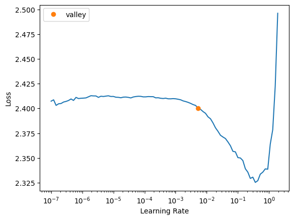
learn.lr_find()

SuggestedLRs(valley=0.005248074419796467)

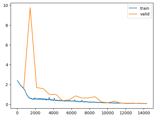
learn.fit_one_cycle(20, lr_max=2e-2)

epoch	train_loss	valid_loss	custom_f1	time
0	1.589015	1.613296	0.430276	00:08
1	0.596273	9.769330	0.138490	00:08
2	0.536909	1.681139	0.506053	00:08
3	0.539270	1.579196	0.548123	00:08
4	0.512807	0.979058	0.691534	00:08
5	0.392594	0.993256	0.706776	00:08
6	0.330091	0.355182	0.913945	00:08
7	0.342943	0.441820	0.862817	00:08
8	0.306386	0.845925	0.716009	00:08
9	0.374366	0.628933	0.800235	00:08
10	0.223469	0.635979	0.808553	00:08
11	0.193208	0.762577	0.776152	00:08
12	0.167112	0.234091	0.938420	00:08
13	0.145844	0.152724	0.961894	00:08
14	0.122106	0.298447	0.915034	00:08
15	0.130290	0.112660	0.972302	00:08
16	0.089869	0.104017	0.975089	00:08
17	0.088174	0.088870	0.978922	00:08
18	0.080296	0.070198	0.985541	00:08
19	0.073266	0.068224	0.985759	00:08

learn.recorder.plot_loss()

learn.model.eval()

RNN(
  (encoder): Embedding(11, 5)
  (rnns): ModuleList(
    (0): LSTM(5, 7, batch_first=True)
  )
  (linear): LinBnDrop(
    (0): BatchNorm1d(21, eps=1e-05, momentum=0.1, affine=True, track_running_stats=True)
    (1): Linear(in_features=21, out_features=11, bias=False)
  )
)

def predict_numbers(model, prompt, length=1):
    txt = num(tkn(prompt)).unsqueeze(0).to(default_device())
    for _ in range(length - txt.shape[-1]):
        pred = model(txt)
        next_tkn = pred.softmax(1).argmax(1, keepdim=True)
        txt = torch.cat((txt, next_tkn), dim=1)
    return ''.join(num.decodes(txt.squeeze()))

prompt = "119;120;121;122;123;124;12"
predict_numbers(learn.model, prompt, length=30)

'119;120;121;122;123;124;128;;;'

prompt = "5498;5499;5500;5501;5502;"
predict_numbers(learn.model, prompt, length=30)

'5498;5499;5500;5501;5502;21;;;'

prompt = "877777;877778;877779;87"
predict_numbers(learn.model, prompt, length=30)

'877777;877778;877779;87877;;;;'

L(learn.model.encoder.parameters())

(#1) [Parameter containing:
tensor([[-0.2031, -0.1375, -0.2440, -0.1413, -0.3468],
        [-0.2825, -0.1776, -0.0832, -0.1576,  0.2265],
        [ 0.1438,  0.1397, -0.2305, -0.2358,  0.1374],
        [ 0.1390,  0.0155,  0.0616, -0.3062, -0.2401],
        [ 0.0579, -0.0481,  0.3006, -0.1747,  0.1483],
        [ 0.2654,  0.1297,  0.1048,  0.1523,  0.3230],
        [ 0.2667,  0.0638,  0.0783,  0.1076, -0.2055],
        [-0.0081, -0.1284,  0.1845,  0.1414, -0.3178],
        [-0.2606, -0.2595,  0.0815,  0.2693,  0.0481],
        [-0.0115,  0.1620, -0.6675,  0.3785,  0.3471],
        [-0.8454,  0.8503,  0.4260, -0.0279, -0.0558]], device='cuda:0',
       requires_grad=True)]

preds_b = learn.model(xb)

preds_b.argmax(1)

tensor([ 9,  8,  0,  7,  3, 10,  6,  6,  0,  5,  0,  4,  9,  5, 10,  8,  5,  2,
         4,  7,  6,  5,  4,  1,  3,  9,  8,  7,  2, 10, 10,  7,  5,  1,  6,  4,
        10,  5,  1,  0,  8, 10,  8,  6,  5,  2,  0,  9,  6,  7,  9,  8,  0,  7,
         7,  9,  6,  9,  1,  1,  5,  5,  1, 10,  3,  9,  2, 10,  1,  7,  3,  3,
         6,  7,  4,  2,  1,  1,  0,  7,  7,  1,  7,  9,  1,  2,  3,  6,  6,  7,
         9,  1,  5,  9,  0, 10, 10,  7, 10,  6,  3,  8,  2,  5,  5,  3,  1, 10,
         3,  7,  2, 10, 10,  3,  6,  3,  5,  1,  2,  0,  7,  0,  5,  4,  8, 10,
         9,  9], device='cuda:0')

yb

tensor([ 9,  8,  0,  7,  3, 10,  6,  6,  0,  5,  0,  4,  9,  5, 10,  8,  5,  2,
         5,  7,  6,  5,  4,  1,  3,  9,  8,  7,  2, 10, 10,  7,  5,  1,  6,  4,
        10,  3,  1,  0,  8, 10,  8,  6,  5,  2,  0,  9,  6,  7,  9,  8,  0,  7,
         7,  9,  6,  9,  1,  1,  5,  5,  3, 10,  3,  9,  2, 10,  3,  7,  3,  3,
         6,  7,  4,  2,  1,  1,  0,  7,  7,  1,  7,  9,  1,  2,  3,  6,  6,  7,
         9,  1,  5,  9,  0, 10, 10,  7, 10,  6,  3,  8,  2,  5,  5,  3,  1, 10,
         3,  7,  2, 10, 10,  3,  6,  3,  5,  1,  2,  0,  7,  0,  5,  4,  8, 10,
         9,  9], device='cuda:0')

References

Brown, Tom, Benjamin Mann, Nick Ryder, Melanie Subbiah, Jared D Kaplan, Prafulla Dhariwal, Arvind Neelakantan, et al. 2020. “Language Models Are Few-Shot Learners.” In Advances in Neural Information Processing Systems, edited by H. Larochelle, M. Ranzato, R. Hadsell, M. F. Balcan, and H. Lin, 33:1877–1901. Curran Associates, Inc. https://proceedings.neurips.cc/paper/2020/file/1457c0d6bfcb4967418bfb8ac142f64a-Paper.pdf.

Caron, Mathilde, Hugo Touvron, Ishan Misra, Hervé Jégou, Julien Mairal, Piotr Bojanowski, and Armand Joulin. 2021. “Emerging Properties in Self-Supervised Vision Transformers.” In Proceedings of the IEEE/CVF International Conference on Computer Vision (ICCV), 9650–60. https://doi.org/10.1109/ICCV48922.2021.00951.

Iten, Raban, Tony Metger, Henrik Wilming, Lı́dia Del Rio, and Renato Renner. 2020. “Discovering Physical Concepts with Neural Networks.” Phys. Rev. Lett. 124 (1): 010508. https://doi.org/10.1103/PhysRevLett.124.010508.

Kottmann, Korbinian, Patrick Huembeli, Maciej Lewenstein, and Antonio Acı́n. 2020. “Unsupervised Phase Discovery with Deep Anomaly Detection.” Phys. Rev. Lett. 125 (October): 170603. https://doi.org/10.1103/PhysRevLett.125.170603.